from aff_poly_sig.exp_sig import expsig, withwords, expsig_withwords, momentsAffine and polynomial methods for signatures
Code for Laplace transform of the signature of a one dimensional Brownian motion and expected signature of a continuous polynomial process.
Documentation
The code documentation is available at https://sarasvaluto.github.io/AffPolySig/.
The original theoretical results can be found in the following papers.
C. Cuchiero, G. Gazzani, J. Möller, and S. Svaluto-Ferro. Joint calibration to SPX and VIX options with signature-based models. ArXiv e-prints, 2023. https://arxiv.org/abs/2301.13235.
C. Cuchiero, S. Svaluto-Ferro, and J. Teichmann. Signature SDEs from an affine and polynomial perspectiv. ArXiv e-prints, 2023. http://arxiv.org/abs/2302.01362
How to install
After cloning the repository, cd (change directory) to the repo and enter this into your terminal:
pip install -e .How to use
Expected signature and moments of a polynomial process
The goal of this code is to compute the expected signature \(\mathbb E[\mathbb X_T]\) of a polynomial process \(X\). In the one dimensional case it also provides an expression for its moments. As a first step import the following functions.
Next, define the parameters of the polynomial process of interest. Given the drift vector \[b(X_t)^i=b_i+\sum_{j=0}^db_{ij}X_t^j,\] and the diffusion matrix \[a(X_t)^{ij}=a_{ij}+\sum_{k=0}^da_{ijk}X_t^k+\sum_{k,h=0}^da_{ijkh}X_t^kX_t^h,\] we use the following parametrisation of the characteristics \[\begin{align*} b_{const}[i]&=b_i,& b_{lin}[i,j]&=b_{ij},\\ a_{const}[i,j]&=a_{ij},& a_{lin}[i,j,k]&=a_{ijk},& a_{quad}[i,j,k,h]=a_{ijkh}. \end{align*}\] Coefficients need then to be saved in a tuple as illustrated in the code below. Define also the initial condition \(x_0\).
For this example we consider a one dimensional Jacobi process without drift setting \(b(X_t)^0=0\) and \(a(X_t)^{00}=X_t^0(1-X_t)^0\). We set \(x_0=1/2\).
import numpy as np

#Dimension of the process
dim=1

#Coefficients of the characteristics
b_const=np.zeros(dim)
b_lin=np.zeros((dim,dim))
a_const=np.zeros((dim,dim))
a_lin=np.zeros((dim,dim,dim))
a_quad=np.zeros((dim,dim,dim,dim))

a_lin[0]=1
a_quad[0]=-1

coeff=(b_const,b_lin,a_const,a_lin,a_quad)

x0=np.zeros(dim)
x0[0]=1/2
The last parameters to define are given by the lenght of the expected signature we would like to compute (len_max) and the time at which we would like to do it (T).
len_max=10
T=1
To get the expected signature we can then use the function expsig.
expsig(coeff,x0,len_max,dim,T)array([1.00000000e+00, 0.00000000e+00, 7.90150699e-02, 0.00000000e+00,
1.45583443e-03, 0.00000000e+00, 1.14548260e-05, 0.00000000e+00,
4.94622744e-08, 0.00000000e+00, 1.34438690e-10])To obtain a better readable output one can use the function withwords.
E=expsig(coeff,x0,len_max,dim,T)
withwords(E,dim)
[[1.0, []],
[0.07901506985356974, [0, 0]],
[0.0014558344297645905, [0, 0, 0, 0]],
[1.145482602482784e-05, [0, 0, 0, 0, 0, 0]],
[4.94622743536099e-08, [0, 0, 0, 0, 0, 0, 0, 0]],
[1.3443868989326117e-10, [0, 0, 0, 0, 0, 0, 0, 0, 0, 0]]]The same result can be obtained directly using expsig_withwords, which combines the two steps above.
expsig_withwords(coeff,x0,len_max,dim,T)[[1.0, []],
[0.07901506985356974, [0, 0]],
[0.0014558344297645905, [0, 0, 0, 0]],
[1.145482602482784e-05, [0, 0, 0, 0, 0, 0]],
[4.94622743536099e-08, [0, 0, 0, 0, 0, 0, 0, 0]],
[1.3443868989326117e-10, [0, 0, 0, 0, 0, 0, 0, 0, 0, 0]]]In one dimension (dim=1) we can also use the function moments to compute the moments of the process.
moments(coeff,x0,len_max,dim,T)array([1. , 0.5 , 0.40803014, 0.36204521, 0.33448524,
0.31613774, 0.30305083, 0.29324856, 0.28563369, 0.27954838,
0.2745743 ])Laplace transform in the Brownian setting
The goal of this code is to compute the Laplace transform \(\mathbb E[e^{\langle \mathbf u^{sig}, \mathbb X_t^{sig}\rangle}]\) and \(\mathbb E[e^{\langle \mathbf u^{pow}, \mathbb X_t^{pow}\rangle}]\), where \(X\) denotes a Brownian motion and \(\mathbb X^{sig}\) and \(\mathbb X^{pow}\) the corresponding extensions. Precisely, we consider the following two extensions: the signature \[\mathbb X_t^{sig}:=(1,X_t,\frac {X_t^2}2,\ldots),\] and the power sequence \[\mathbb X_t^{pow}:=(1,X_t,X_t^2,\ldots).\] As a first step import the following functions.
from aff_poly_sig.riccati_bm import appr_exp_sig, appr_exp_pow, MC, CoDNext, we introduce the parameters of interest. We in particular have T for the time horizon, K_u for the lenght of (the approximation of) \(\mathbf u^{sig}\) and \(\mathbf u^{pow}\), u_sig for \(\mathbf u^{sig}\) with the signature’s extension, and u_pow for \(\mathbf u^{pow}\) with the power sequence’s extension. As an example we compute \[\mathbb E[\exp(-2\frac{X_t^2}2)]=\mathbb E[\exp(-X_t^2)]\] for each \(t\in[0,T]\), where \(X\) denotes a Brownian Motion and \(T=1\). The corresponding parameters are given in the following cell.
import math
import matplotlib.pyplot as plt

T=1 # [0,T] time horizon

#u in terms of the sig lift
K_u=5
u_sig=np.zeros(K_u)
u_sig[2]=-2

#u in terms of the powers lift
u_pow=u_sig.copy()
for k in range(0,K_u):
    u_pow[k]=u_pow[k]/math.factorial(k)
One then just needs to fix the computational parameters, namely the grid for the computation of the signature (timegrid) and the trucation’s level K for the solution.
n_time=1000
timegrid = np.linspace(0,T,n_time)
K=30
The desired Laplace transform can then be computed using appr_exp_sig and appr_exp_pow. The finals sig and pow denote the employed extensions.
L_sig=appr_exp_sig(u_sig,timegrid,K)
L_pow=appr_exp_pow(u_pow,timegrid,K)
To test the results, one can compare them to the results obtained by a Monte Carlo approximation. That’s what the MC function does.
N=100000 # number of samples
n_MC=1000 # number of times ticks
MonteCarlo = MC(u_sig,T,n_MC,N)
#Monte Carlo
#MonteCarlo_CoD = CoD(np.real(MonteCarlo),n_MC, n_time)
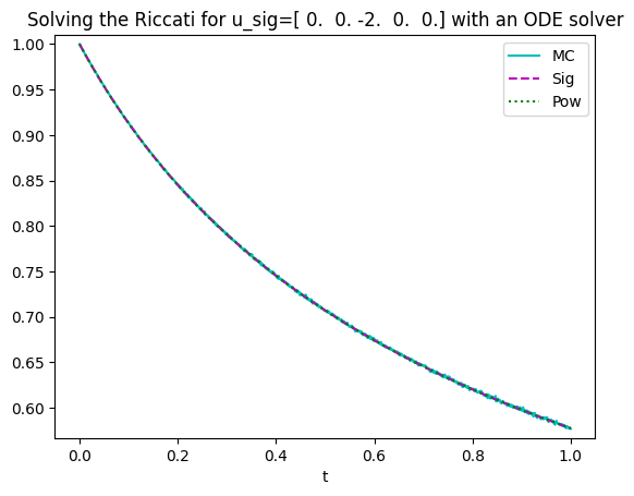
plt.plot(np.linspace(0,T,n_MC),MonteCarlo,'c',label='MC');
#Sig Lift
plt.plot(timegrid,L_sig,'m--',label='Sig');
#Pow Lift
plt.plot(timegrid,L_pow,'g:',label='Pow');
plt.ylim(min(MonteCarlo.real-0.01),max(MonteCarlo.real)+0.01)
plt.xlabel("t")
plt.title(f'Solving the Riccati for u_sig={u_sig.real} with an ODE solver')
plt.legend();